Plot multi-class SGD on the iris dataset

Plot decision surface of multi-class SGD on iris dataset. The hyperplanes corresponding to the three one-versus-all (OVA) classifiers are represented by the dashed lines.

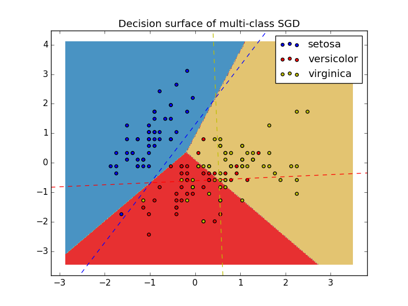
Python source code: plot_sgd_iris.py

print(__doc__)

import numpy as np
import matplotlib.pyplot as plt
from sklearn import datasets
from sklearn.linear_model import SGDClassifier

# import some data to play with
iris = datasets.load_iris()
X = iris.data[:, :2]  # we only take the first two features. We could
                      # avoid this ugly slicing by using a two-dim dataset
y = iris.target
colors = "bry"

# shuffle
idx = np.arange(X.shape[0])
np.random.seed(13)
np.random.shuffle(idx)
X = X[idx]
y = y[idx]

# standardize
mean = X.mean(axis=0)
std = X.std(axis=0)
X = (X - mean) / std

h = .02  # step size in the mesh

clf = SGDClassifier(alpha=0.001, n_iter=100).fit(X, y)

# create a mesh to plot in
x_min, x_max = X[:, 0].min() - 1, X[:, 0].max() + 1
y_min, y_max = X[:, 1].min() - 1, X[:, 1].max() + 1
xx, yy = np.meshgrid(np.arange(x_min, x_max, h),
                     np.arange(y_min, y_max, h))

# Plot the decision boundary. For that, we will assign a color to each
# point in the mesh [x_min, m_max]x[y_min, y_max].
Z = clf.predict(np.c_[xx.ravel(), yy.ravel()])
# Put the result into a color plot
Z = Z.reshape(xx.shape)
cs = plt.contourf(xx, yy, Z, cmap=plt.cm.Paired)
plt.axis('tight')

# Plot also the training points
for i, color in zip(clf.classes_, colors):
    idx = np.where(y == i)
    plt.scatter(X[idx, 0], X[idx, 1], c=color, label=iris.target_names[i],
                cmap=plt.cm.Paired)
plt.title("Decision surface of multi-class SGD")
plt.axis('tight')

# Plot the three one-against-all classifiers
xmin, xmax = plt.xlim()
ymin, ymax = plt.ylim()
coef = clf.coef_
intercept = clf.intercept_


def plot_hyperplane(c, color):
    def line(x0):
        return (-(x0 * coef[c, 0]) - intercept[c]) / coef[c, 1]

    plt.plot([xmin, xmax], [line(xmin), line(xmax)],
             ls="--", color=color)

for i, color in zip(clf.classes_, colors):
    plot_hyperplane(i, color)
plt.legend()
plt.show()

Total running time of the example: 0.20 seconds ( 0 minutes 0.20 seconds)