
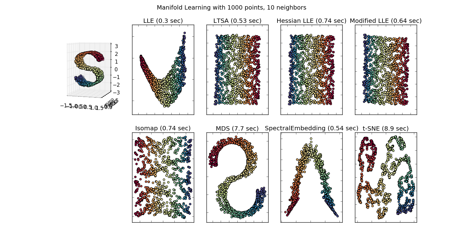
Comparison of Manifold Learning methods
An illustration of dimensionality reduction on the S-curve dataset with various manifold learning methods.
For a discussion and comparison of these algorithms, see the manifold module page
For a similar example, where the methods are applied to a sphere dataset, see Manifold Learning methods on a severed sphere
Note that the purpose of the MDS is to find a low-dimensional representation of the data (here 2D) in which the distances respect well the distances in the original high-dimensional space, unlike other manifold-learning algorithms, it does not seeks an isotropic representation of the data in the low-dimensional space.
Script output:
standard: 0.3 sec
ltsa: 0.53 sec
hessian: 0.74 sec
modified: 0.64 sec
Isomap: 0.74 sec
MDS: 7.7 sec
SpectralEmbedding: 0.54 sec
t-SNE: 8.9 sec
Python source code: plot_compare_methods.py
# Author: Jake Vanderplas -- <vanderplas@astro.washington.edu>

print(__doc__)

from time import time

import matplotlib.pyplot as plt
from mpl_toolkits.mplot3d import Axes3D
from matplotlib.ticker import NullFormatter

from sklearn import manifold, datasets

# Next line to silence pyflakes. This import is needed.
Axes3D

n_points = 1000
X, color = datasets.samples_generator.make_s_curve(n_points, random_state=0)
n_neighbors = 10
n_components = 2

fig = plt.figure(figsize=(15, 8))
plt.suptitle("Manifold Learning with %i points, %i neighbors"
             % (1000, n_neighbors), fontsize=14)

try:
    # compatibility matplotlib < 1.0
    ax = fig.add_subplot(251, projection='3d')
    ax.scatter(X[:, 0], X[:, 1], X[:, 2], c=color, cmap=plt.cm.Spectral)
    ax.view_init(4, -72)
except:
    ax = fig.add_subplot(251, projection='3d')
    plt.scatter(X[:, 0], X[:, 2], c=color, cmap=plt.cm.Spectral)

methods = ['standard', 'ltsa', 'hessian', 'modified']
labels = ['LLE', 'LTSA', 'Hessian LLE', 'Modified LLE']

for i, method in enumerate(methods):
    t0 = time()
    Y = manifold.LocallyLinearEmbedding(n_neighbors, n_components,
                                        eigen_solver='auto',
                                        method=method).fit_transform(X)
    t1 = time()
    print("%s: %.2g sec" % (methods[i], t1 - t0))

    ax = fig.add_subplot(252 + i)
    plt.scatter(Y[:, 0], Y[:, 1], c=color, cmap=plt.cm.Spectral)
    plt.title("%s (%.2g sec)" % (labels[i], t1 - t0))
    ax.xaxis.set_major_formatter(NullFormatter())
    ax.yaxis.set_major_formatter(NullFormatter())
    plt.axis('tight')

t0 = time()
Y = manifold.Isomap(n_neighbors, n_components).fit_transform(X)
t1 = time()
print("Isomap: %.2g sec" % (t1 - t0))
ax = fig.add_subplot(257)
plt.scatter(Y[:, 0], Y[:, 1], c=color, cmap=plt.cm.Spectral)
plt.title("Isomap (%.2g sec)" % (t1 - t0))
ax.xaxis.set_major_formatter(NullFormatter())
ax.yaxis.set_major_formatter(NullFormatter())
plt.axis('tight')


t0 = time()
mds = manifold.MDS(n_components, max_iter=100, n_init=1)
Y = mds.fit_transform(X)
t1 = time()
print("MDS: %.2g sec" % (t1 - t0))
ax = fig.add_subplot(258)
plt.scatter(Y[:, 0], Y[:, 1], c=color, cmap=plt.cm.Spectral)
plt.title("MDS (%.2g sec)" % (t1 - t0))
ax.xaxis.set_major_formatter(NullFormatter())
ax.yaxis.set_major_formatter(NullFormatter())
plt.axis('tight')


t0 = time()
se = manifold.SpectralEmbedding(n_components=n_components,
                                n_neighbors=n_neighbors)
Y = se.fit_transform(X)
t1 = time()
print("SpectralEmbedding: %.2g sec" % (t1 - t0))
ax = fig.add_subplot(259)
plt.scatter(Y[:, 0], Y[:, 1], c=color, cmap=plt.cm.Spectral)
plt.title("SpectralEmbedding (%.2g sec)" % (t1 - t0))
ax.xaxis.set_major_formatter(NullFormatter())
ax.yaxis.set_major_formatter(NullFormatter())
plt.axis('tight')

t0 = time()
tsne = manifold.TSNE(n_components=n_components, init='pca', random_state=0)
Y = tsne.fit_transform(X)
t1 = time()
print("t-SNE: %.2g sec" % (t1 - t0))
ax = fig.add_subplot(2, 5, 10)
plt.scatter(Y[:, 0], Y[:, 1], c=color, cmap=plt.cm.Spectral)
plt.title("t-SNE (%.2g sec)" % (t1 - t0))
ax.xaxis.set_major_formatter(NullFormatter())
ax.yaxis.set_major_formatter(NullFormatter())
plt.axis('tight')

plt.show()
Total running time of the example: 21.09 seconds ( 0 minutes 21.09 seconds)