Deep Metric Learning
- Introduction
- Related works
- Review
- Deep metric learning via lifted structured feature embedding
- Implementation details
- Evaluation
- Experiments
- Conclusion
(CVPR 2016) Deep Metric Learning via Lifted Structured Feature Embedding
Project Page: http://cvgl.stanford.edu/projects/lifted_struct/
Code: https://github.com/rksltnl/Deep-Metric-Learning-CVPR16
In this paper, we describe an algorithm for taking full advantage of the training batches in the neural network training by lifting the vector of pairwise distances within the batch to the matrix of pairwise distances.
Additionally, we collected Online Products dataset: 120k images of 23k classes of online products for metric learning.
Introduction
Given such a similarity function, classification tasks could be simply reduced to the nearest neighbor problem with the given similarity measure, and clustering tasks would be made easier given the similarity matrix.
extreme classification:
algorithms with the learning and inference complexity linear in the number of classes become impractical.
the availability of training data per class becomes very scarce.
However, the existing approaches [1, 31] cannot take full advantage of the training batches used during the mini batch stochastic gradient descent training of the networks [20, 33].
Our proposed method lifts the vector of pairwise distances \((O(m))\) within the batch to the matrix of pairwise distances \((O(m^2))\). Then we design a novel structured loss objective on the lifted problem.
We evaluate our methods on the CUB200-2011 [37], CARS196 [19], and Online Products dataset we collected. The Online Products has approximately 120k images and 23k classes of product photos from online e-commerce websites.
Related works
Deep metric learning
Deep feature embedding with state of the art convolutional neural networks
Zero shot learning and ranking
Review
Contrastive embedding [14] is trained on the paired data \(\{(x_i, x_j, y_{ij})\}\). Intuitively, the contrastive training minimizes the distance between a pair of examples with the same class label and penalizes the negative pair distances for being smaller than the margin parameter \(\alpha\).
\[J = \frac{1}{m} \sum_{(i,j)}^{m/2} y_{i,j} D_{i,j}^2 + (1 - y_{i,j})[\alpha - D_{i,j}]_+^2\]
where \(m\) stands for the number of images in the batch, \(f(·)\) is the feature embedding output from the network, \(D_{i,j} = \lVert f(x_i) − f(x_j) \rVert_2\), and the label \(y_{i,j} \in \{0, 1\}\) indicates whether a pair \((x_i, x_j)\) is from the same class or not. The \([·]_+\) operation indicates the hinge function \(\max(0, ·)\).
Triplet embedding [39, 31] is trained on the triplet data \(\{(x_a^{(i)}, x_p^{(i)}, x_n^{(i)})\}\) where \((x_a^{(i)}, x_p^{(i)})\) have the same class labels and \((x_a^{(i)}, x_n^{(i)})\) have different class labels. The \(x_a^{(i)}\) term is referred to as an anchor of a triplet. Intuitively, the training process encourages the network to find an embedding where the distance between \(x_a^{(i)}\) and \(x_n^{(i)}\) is larger than the distance between \(x_a^{(i)}\) and \(x_p^{(i)}\) plus the margin parameter \(\alpha\).
\[J = \frac{3}{2m} \sum_i^{m/3} [D_{ia, ip}^2 - D_{ia, in}^2 + \alpha]_+\]
where \(D_{ia, ip} = \lVert f(x_i^a) − f(x_i^p) \rVert\) and \(D_{ia, in} = \lVert f(x_i^a) − f(x_i^n) \rVert\).
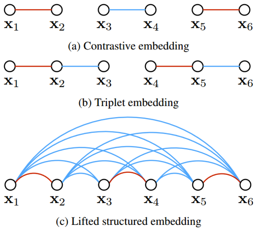
Figure 2: Illustration for a training batch with six examples. Red edges and blue edges represent similar and dissimilar examples respectively. In contrast, our method explicitly takes into account all pair wise edges within the batch.
Deep metric learning via lifted structured feature embedding
We define a structured loss function based on all positive and negative pairs of samples in the training set:
\[J = \frac{1}{2 \lvert \hat{P} \rvert} \sum_{(i, j) \in \hat{P}} \max (0, J_{i, j})^2\]
\[J_{i, j} = \max ( \max_{(i, k) \in \hat{N}} \alpha - D_{i, k}, \max_{(j, l) \in \hat{N}} \alpha - D_{j, l} ) + D_{i, j}\]
where \(\hat{P}\) is the set of positive pairs and \(\hat{N}\) is the set of negative pairs in the training set.
This function poses two computational challenges:
it is non-smooth,
both evaluating it and computing the subgradient requires mining all pairs of examples several times.
We address these challenges in two ways:
we optimize a smooth upper bound on the function instead.
as is common for large data sets, we use a stochastic approach.
we change our batch to be not completely random, but integrate elements of importance sampling. We
sample a few positive pairs at random, and then actively add their difficult neighbors to the training mini-batch.
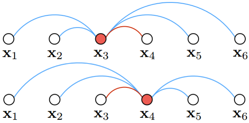
Figure 4: Hard negative edge is mined with respect to each left and right example per each positive pairs. In this illustration with 6 examples in the batch, both x3 and x4 independently compares against all other negative edges and mines the hardest negative edge.
mining the single hardest negative with nested max functions (eqn. 4) in practice causes the network to converge to a bad local optimum. Hence we optimize the following smooth upper bound \(\tilde{J}(D(f(x)))\).
\[\tilde{J}_{i, j} = \log ( \sum_{(i, k) \in N} \exp \{\alpha - D_{i, k}\} + \sum_{(j, l) \in N} \exp \{\alpha - D_{j, l}\} ) + D_{i, j}\]
\[\tilde{J} = \frac{1}{2 \lvert P \rvert} \sum_{(i, j) \in P} \max (0, \tilde{J}_{i, j})^2\]
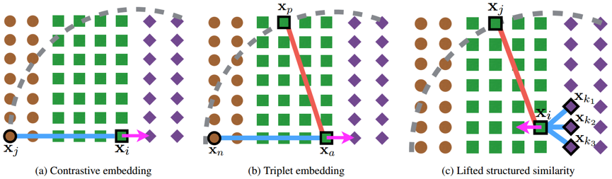
Figure 5: Illustration of failure modes of contrastive and triplet loss with randomly sampled training batch. Brown circles, green squares, and purple diamonds represent three different classes. Dotted gray arcs indicate the margin bound (where the loss becomes zero out of the bound) in the hinge loss. Magenta arrows denote the negative gradient direction for the positives.
Implementation details
We used the Caffe [16] package for training and testing the embedding with contrastive [14], triplet [31, 39], and ours. Maximum training iteration was set to 20000 for all the experiments. The margin parameter \(\alpha\) was set to 1.0. The batch size was set to 128 for contrastive and our method and to 120 for triplet.
Evaluation
For the clustering task, we use the \(F_1\) and NMI metrics.
\(F_1\) metric computes the harmonic mean of precision and recall.
Normalized mutual information (NMI) is defined by the ratio of mutual information and the average entropy of clusters and the entropy of labels.
For the retrieval task, we use the Recall@K [15] metric.
Each test image (query) first retrieves K nearest neighbors from the test set and receives score 1 if an image of the same class is retrieved among the K nearest neighbors and 0 otherwise. Recall@K averages this score over all the images.
Experiments
CUB-200-2011
The CUB-200-2011 dataset [37] has 200 classes of birds with 11,788 images. We split the first 100 classes for training (5,864 images) and the rest of the classes for testing (5,924 images).
CARS196
The CARS196 data set [19] has 198 classes of cars with 16,185 images. We split the first 98 classes for training (8,054 images) and the other 98 classes for testing (8,131 images).
Online Products dataset
We used the web crawling API from eBay.com [9] to download images and filtered duplicate and irrelevant images (i.e. photos of contact phone numbers, logos, etc). The preprocessed dataset has 120,053 images of 22,634 online products (classes) from eBay.com. Each product has approximately 5:3 images. For the experiments, we split 59,551 images of 11,318 classes for training and 60,502 images of 11,316 classes for testing.
Conclusion
We described a deep feature embedding and metric learning algorithm which defines a novel structured prediction objective on the lifted dense pairwise distance matrix within the batch during the neural network training.