ENet
ENet: A Deep Neural Network Architecture for Real-Time Semantic Segmentation
Paper: https://arxiv.org/abs/1606.02147
Code: https://github.com/e-lab/ENet-training
提出一种做语义分割的速度快且准确率不低的网络ENet。
ENet采用类似ResNet的bottleneck模块:模块包含3个卷积层(1x1投影降维,主卷积层,1x1扩张),卷积之间添加BN层和PReLU。
下采样会丢失边缘信息,上采样计算量大,但下采样会有更大的感受野,更多上下文信息。综合考虑,使用dilated convolutions。
输入大图耗时间,故前两个block就下采样保留少量feature map去除图片中冗余部分。
采用大encoder,小decoder。
采用ReLU反而降低精度,可能因为层数较少。
维度下降容易丢失信息,故与stride=2的卷积并行进行pooling最后合并得到feature map。这样比原来的block快10倍。
卷积权重有冗余,把\(n \times n\)的卷积分解成\(n \times 1\)和\(1 \times n\)的小卷积。
使用Spatial Dropout提高准确率。
we propose a novel deep neural network architecture named ENet (efficient neural network), created specifically for tasks requiring low latency operation.
Introduction
These references propose networks with huge numbers of parameters, and long inference times.
we propose a new neural network architecture optimized for fast inference and high accuracy.
Related work
However, these networks are slow during inference due to their large architectures and numerous parameters.
Unlike in fully convolutional networks (FCN) [12], fully connected layers of VGG16 were discarded in the latest incarnation of SegNet, in order to reduce the number of floating point operations and memory footprint, making it the smallest of these networks.
Network architecture
We adopt a view of ResNets [24] that describes them as having a single main branch and extensions with convolutional filters that separate from it, and then merge back with an element-wise addition, as shown in Figure 2b.
Each block consists of three convolutional layers: a \(1 \times 1\) projection that reduces the dimensionality, a main convolutional layer (conv in Figure 2b), and a \(1 \times 1\) expansion. We place Batch Normalization [25] and PReLU [26] between all convolutions.
Just as in the original paper, we refer to these as bottleneck modules.
If the bottleneck is downsampling, a max pooling layer is added to the main branch.
Also, the first \(1 \times 1\) projection is replaced with a \(2 \times 2\) convolution with stride 2 in both dimensions.
We zero pad the activations, to match the number of feature maps.
conv is either a regular, dilated or full convolution (also known as deconvolution or fractionally strided convolution) with \(3 \times 3\) filters.
Sometimes we replace it with asymmetric convolution i.e. a sequence of \(5 \times 1\) and \(1 \times 5\) convolutions.
For the regularizer, we use Spatial Dropout [27], with \(p = 0.01\) before bottleneck2.0, and \(p = 0.1\) afterwards.
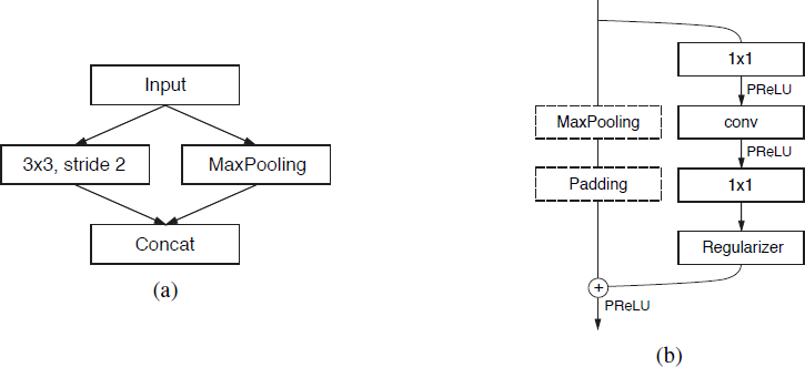
Figure 2: (a) ENet initial block. MaxPooling is performed with non-overlapping \(2 \times 2\) windows, and the convolution has 13 filters, which sums up to 16 feature maps after concatenation. This is heavily inspired by [28]. (b) ENet bottleneck module. conv is either a regular, dilated, or full convolution (also known as deconvolution) with \(3 \times 3\) filters, or a \(5 \times 5\) convolution decomposed into two asymmetric ones.
The initial stage contains a single block, that is presented in Figure 2a.
Stage 1 consists of 5 bottleneck blocks, while stage 2 and 3 have the same structure, with the exception that stage 3 does not downsample the input at the beginning (we omit the 0th bottleneck).
These three first stages are the encoder.
Stage 4 and 5 belong to the decoder.
In the decoder max pooling is replaced with max unpooling, and padding is replaced with spatial convolution without bias.
for performance reasons, we decided to place only a bare full convolution as the last module of the network.
Design choices
Feature map resolution
Downsampling images during semantic segmentation has two main drawbacks.
reducing feature map resolution implies loss of spatial information like exact edge shape.
full pixel segmentation requires that the output has the same resolution as the input.
The first issue has been addressed in FCN [12] by adding the feature maps produced by encoder, and in SegNet [10] by saving indices of elements chosen in max-pooling layers, and using them to produce sparse upsampled maps in the decoder. We followed the SegNet approach, because it allows to reduce memory requirements.
downsampling has one big advantage. Filters operating on downsampled images have a bigger receptive field, that allows them to gather more context.
In the end, we have found that it is better to use dilated convolutions for this purpose [30].
Early downsampling
processing large input frames is very expensive.
ENet first two blocks heavily reduce the input size, and use only a small set of feature maps.
visual information is highly spatially redundant.
our intuition is that the initial network layers should not directly contribute to classification.
Decoder size
our architecture consists of a large encoder, and a small decoder.
Nonlinear operations
we have found that removing most ReLUs in the initial layers of the network improved the results.
We replaced all ReLUs in the network with PReLUs [26], which use an additional parameter per feature map, with the goal of learning the negative slope of non-linearities.
Initial layers weights exhibit a large variance and are slightly biased towards positive values, while in the later portions of the encoder they settle to a recurring pattern. All layers in the main branch behave nearly exactly like regular ReLUs, while the weights inside bottleneck modules are negative i.e. the function inverts and scales down negative values.
the decoder weights become much more positive and learn functions closer to identity.
Information-preserving dimensionality changes
but aggressive dimensionality reduction can also hinder the information flow.
introduces a representational bottleneck (or forces one to use a greater number of filters, which lowers computational efficiency).
as proposed in [28], we chose to perform pooling operation in parallel with a convolution of stride 2, and concatenate resulting feature maps.
This technique allowed us to speed up inference time of the initial block 10 times.
Additionally, we have found one problem in the original ResNet architecture. When downsampling, the first \(1 \times 1\) projection of the convolutional branch is performed with a stride of 2 in both dimensions, which effectively discards 75% of the input.
Increasing the filter size to \(2 \times 2\) allows to take the full input into consideration, and thus improves the information flow and accuracy.
Factorizing filters
convolutional weights have a fair amount of redundancy
each \(n \times n\) convolution can be decomposed into two smaller ones following each other: one with a \(n \times 1\) filter and the other with a \(1 \times n\) filter [32].
refer to these as asymmetric convolutions.
increase the variety of functions learned by blocks and increase the receptive field.
a sequence of operations used in the bottleneck module (projection, convolution, projection) can be seen as decomposing one large convolutional layer into a series of smaller and simpler operations, that are its low-rank approximation.
Dilated convolutions
They replaced the main convolutional layers inside several bottleneck modules in the stages that operate on the smallest resolutions. These gave a significant accuracy boost, by raising IoU on Cityscapes by around 4 percentage points, with no additional cost.
Regularization
We placed Spatial Dropout at the end of convolutional branches, right before the addition, and it turned out to work much better than stochastic depth.
Results
Performance Analysis
For inference we merge batch normalization and dropout layers into the convolutional filters, to speed up all networks.
Inference time
Table 2: Performance comparison.
NVIDIA TX1
| Model | 480×320 | 640×360 | 1280×720 |
|---|---|---|---|
| SegNet | 757 ms, 1.3 fps | 1251 ms, 0.8 fps | - ms, - fps |
| ENet | 47 ms, 21.1 fps | 69 ms, 14.6 fps | 262 ms, 3.8 fps |
NVIDIA Titan X
| Model | 640×360 | 1280×720 | 1920×1080 |
|---|---|---|---|
| SegNet | 69 ms, 14.6 fps | 289 ms, 3.5 fps | 637 ms, 1.6 fps |
| ENet | 7 ms, 135.4 fps | 21 ms, 46.8 fps | 46 ms, 21.6 fps |
Table 2 compares inference time for a single input frame of varying resolution. We also report the number of frames per second that can be processed. Dashes indicate that we could not obtain a measurement, due to lack of memory.
Hardware requirements
Table 3: Hardware requirements. FLOPs are estimated for an input of 3 × 640 × 360.
| Model | GFLOPs | Parameters | Model size (fp16) |
|---|---|---|---|
| SegNet | 286.03 | 29.46M | 56.2 MB |
| ENet | 3.83 | 0.37M | 0.7 MB |
Please note that we report storage required to save model parameters in half precision floating point format.
Software limitations
Although applying this method allowed us to greatly reduce the number of floating point operations and parameters, it also increased the number of individual kernels calls, making each of them smaller.
This means that using a higher number of kernels, increases the number of memory transactions, because feature maps have to be constantly saved and reloaded.
We have found that some of these operations can become so cheap, that the cost of GPU kernel launch starts to outweigh the cost of the actual computation.
This means that using a higher number of kernels, increases the number of memory transactions, because feature maps have to be constantly saved and reloaded.
In ENet, PReLUs consume more than a quarter of inference time. Since they are only simple point-wise operations and are very easy to parallelize, we hypothesize it is caused by the aforementioned data movement.
Benchmarks
We have used the Adam optimization algorithm [35] to train the network.
It allowed ENet to converge very quickly and on every dataset we have used training took only 3-6 hours, using four Titan X GPUs.
It was performed in two stages: first we trained only the encoder to categorize downsampled regions of the input image, then we appended the decoder and trained the network to perform upsampling and pixel-wise classification.
Cityscapes
consists of 5000 fine-annotated images
train/val/test: 2975/500/1525
We trained on 19 classes that have been selected in the official evaluation scripts
CamVid
train/test: 367/233
SUN RGB-D
train/test: 5285/5050
37 indoor object classes.
Conclusion
We have proposed a novel neural network architecture designed from the ground up specifically for semantic segmentation. Our main aim is to make efficient use of scarce resources available on embedded platforms, compared to fully fledged deep learning workstations.