SDS
(ECCV 2014) Simultaneous Detection and Segmentation
Paper: https://people.eecs.berkeley.edu/~rbg/papers/BharathECCV2014.pdf
Project Page: https://www2.eecs.berkeley.edu/Research/Projects/CS/vision/shape/sds/
Code: https://github.com/bharath272/sds_eccv2014
We build on recent work that uses convolutional neural networks to classify category-independent region proposals (R-CNN), introducing a novel architecture tailored for SDS. We then use category-specific, top-
down figure-ground predictions to refine our bottom-up proposals.
Introduction
the detected objects are very coarsely localized using just bounding boxes.
A typical semantic segmentation algorithm might accurately mark out the dog pixels in the image, but would provide no indication of how many dogs there are, or of the precise spatial extent of any one particular dog.
The Simultaneous Detection and Segmentation (SDS) algorithm we propose has the following steps:
Proposal generation: use MCG [1] to generate 2000 region candidates per image.
Feature extraction: use a convolutional neural network to extract features on each region. follows work by Girshick et al. [16] (R-CNN).
Region classification: train an SVM on top of the CNN features to assign a score for each category to each candidate.
Region refinement: do non-maximum suppression (NMS) on the scored candidates. then use the features from the CNN to produce category specific coarse mask predictions to refine the surviving candidates.
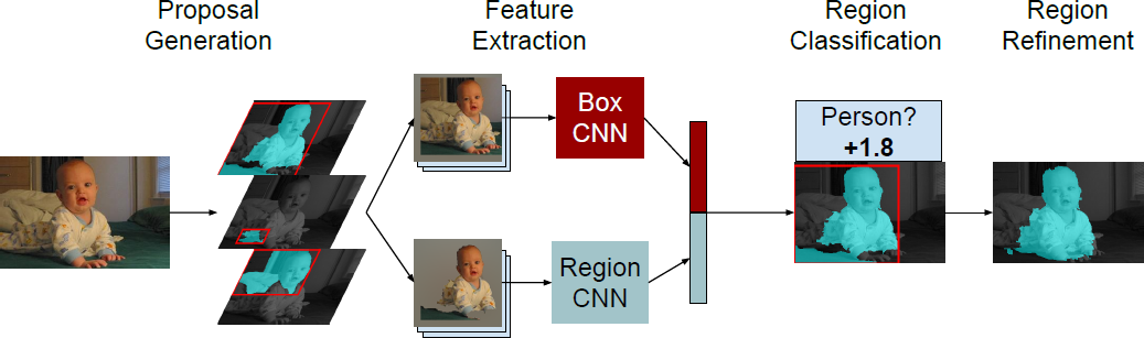
Fig. 1. Overview of our pipeline. Our algorithm is based on classifying region proposals using features extracted from both the bounding box of the region and the region foreground with a jointly trained CNN. A final refinement step improves segmentation.
Given an image, we expect the algorithm to produce a set of object hypotheses, where each hypothesis comes with a predicted segmentation and a score. A hypothesis is correct if its segmentation overlaps with the segmentation of a ground truth instance by more than 50%.
we compute a precision recall (PR) curve, and the average precision (AP), which is the area under the curve. We call the AP computed in this way \(AP^r\) (region, to distinguish it from the traditional bounding box AP, which we call \(AP^b\).
Thus the threshold at which we regard a detection as a true positive depends on the application. As the threshold varies, the PR curve traces out a PR surface. We can use the volume under this PR surface as a metric. We call this metric \(AP^r_vol\) and \(AP^b_{vol}\) respectively.