InstFCN
(ECCV 2016) Instance-sensitive Fully Convolutional Networks
Paper: https://arxiv.org/abs/1603.08678
our FCN is designed to compute a small set of instance-sensitive score maps, each of which is the outcome of a pixel-wise classifier of a relative position to instances.
our method does not have any high-dimensional layer related to the mask resolution, but instead exploits image local coherence for estimating instances.
Introduction
we develop an end-to-end fully convolutional network that is capable of segmenting candidate instances.
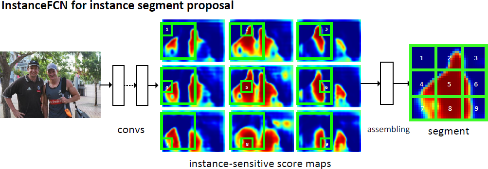
our method computes a set of instance-sensitive score maps, where each pixel is a classifier of relative positions to an object instance.
With this set of score maps, we are able to generate an object instance segment in each sliding window by assembling the output from the score maps.
Unlike DeepMask, our method has no layer whose size is related to the mask size \(m^2\), and each pixel in our method is a low-dimensional classifier. This is made possible by exploiting local coherence [9] of natural images for generating per-window pixel-wise predictions.
Related Work
Instance-sensitive FCNs for Segment Proposal
From FCN to InstanceFCN
the output is indeed reusable for most pixels, except for those where one object is conjunct the other
Instance-sensitive score maps
we propose an FCN where each output pixel is a classifier of relative positions of instances.
In our practice, we define the relative positions using a \(k \times k\) (e.g., \(k = 3\)) regular grid on a square sliding window. We call them instance-sensitive score maps.
Instance assembling module
We slide a window of resolution \(m \times m\) on the set of instance-sensitive score maps. In this sliding window, each \(\frac{m}{k} \times \frac{m}{k}\) sub-window directly copies values from the same sub-window in the corresponding score map. The k2 sub-windows are then put together (according to their relative positions) to assemble a new window of resolution \(m \times m\).
Local Coherence
for a pixel in a natural image, its prediction is most likely the same when evaluated in two neighboring windows.
This allows us to conserve a large number of parameters when the mask resolution \(m^2\) is high.
This not only reduces the computational cost of the mask prediction layers, but more importantly, reduces the number of parameters required for mask regression, leading to less risk of overfitting on small datasets
Algorithm and Implementation
Network architecture
use the VGG-16 network [22] pre-trained on ImageNet [23] as the feature extractor. We follow the practice in [24] to reduce the network stride and increase feature map resolution: the max pooling layer pool4 (between conv4 3 and conv5 1) is modified to have a stride of 1 instead of 2, and accordingly the filters in conv5 1 to conv5 3 are adjusted by the “hole algorithm” [24].
On top of the feature map, there are two fully convolutional branches, one for estimating segment instances and the other for scoring the instances.
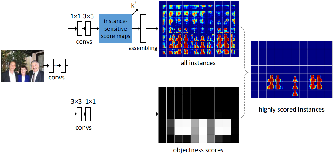
Figure 4. Details of the InstanceFCN architecture. On the top is a fully convolutional branch for generating \(k^2\) instance-sensitive score maps, followed by the assembling module that outputs instances. On the bottom is a fully convolutional branch for predicting the objectness score of each window. The highly scored output instances are on the right. In this figure, the objectness map and the “all instances” map have been sub-sampled for the purpose of illustration.
Training
We adopt the image-centric strategy in [21,19].
The forward pass computes the set of instance-sensitive score maps and the objectness score map.
After that, a set of 256 sliding windows are randomly sampled [21,19], and the instances are only assembled from these 256 windows for computing the loss function.
The loss function is defined as:
\[\sum_i (\mathcal{L}(p_i, p_i^*) + \sum_j \mathcal{L}(S_{i,j}, S_{i,j}^*))\]
Here \(i\) is the index of a sampled window, \(p_i\) is the predicted objectness score of the instance in this window, and \(p_i^*\) is \(1\) if this window is a positive sample and \(0\) if a negative sample. \(S_i\) is the assembled segment instance in this window, \(S_i^*\) is the ground truth segment instance, and \(j\) is the pixel index in the window. \(\mathcal{L}\) is the logistic regression loss.
We follow the scale jittering in [26] for training: a training image is resized such that its shorter side is randomly sampled from \(600 \times 1.5^{ \{−4,−3,−2,−1,0,1\} }\) pixels.
Inference
A forward pass of the network is run on the input image, generating the instance-sensitive score maps and the objectness score map.
The assembling module then applies densely sliding windows on these maps to produce a segment instance at each position.
To handle multiple scales, we resize the shorter side of images to \(600 \times 1.5^{ \{−4,−3,−2,−1,0,1\} }\) pixels, and compute all instances at each scale.
For each output segment, we truncate the values to form a binary mask.
Then we adopt non-maximum suppression (NMS) to generate the final set of segment proposals.
Experiments
Experiments on PASCAL VOC 2012
Ablations on the number of relative positions \(k^2\)
Our method is not sensitive to \(k^2\), and can perform well even when \(k = 3\).
Ablation comparisons with the DeepMask scheme
Comparisons on Instance Semantic Segmentation
Experiments on MS COCO
Conclusion
We have presented InstanceFCN, a fully convolutional scheme for proposing segment instances.
A simple assembling module is then able to generate segment instances from these score maps.
Our network architecture handles instance segmentation without using any high-dimensional layers that depend on the mask resolution.