Semantic Segmentation using Adversarial Networks
- Introduction
- Related Work
- Adversarial training for semantic segmentation networks
- Experimental evaluation results
- Discussion
(NIPS 2016 Workshop) Semantic Segmentation using Adversarial Networks
Paper: https://arxiv.org/abs/1611.08408
we propose an adversarial training approach to train semantic segmentation models.
The motivation for our approach is that it can detect and correct higher-order inconsistencies between ground truth segmentation maps and the ones produced by the segmentation net.
Introduction
Despite many differences in the CNN architectures, a common property across all these approaches is that all label variables are predicted independently from each other.
various post-processing approaches have been explored to reinforce spatial contiguity.
Conditional Markov random fields (CRFs)
Moreover, using a recurrent neural network formulation [30, 35] of the mean-field iterations, it is possible to train the CNN underlying the unary potentials in an integrated manner that takes into account the CRF inference during training.
Higher-order potentials, however, have also been observed to be effective, for example robust higherorder terms based on label consistency across superpixels [13].
We are interested in enforcing higher-order consistency without being limited to a very specific class of high-order potentials.
Contributions:
the first application of adversarial training to semantic segmentation.
The adversarial training approach enforces long-range spatial label contiguity, without adding complexity to the model used at test time.
Our experimental results on the Stanford Background and PASCAL VOC 2012 dataset show that our approach leads to improved labeling accuracy.
Related Work
Adversarial learning
Semantic segmentation
Adversarial training for semantic segmentation networks
Adversarial training
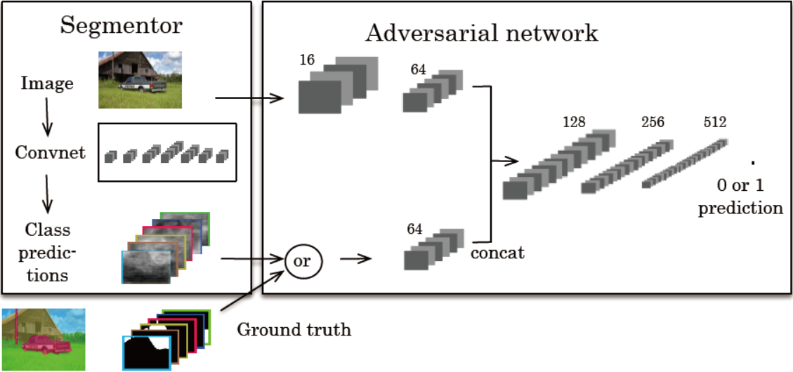
Figure 1: Overview of the proposed approach. Left: segmentation net takes RGB image as input, and produces per-pixel class predictions. Right: Adversarial net takes label map as input and produces class label (1=ground truth, or 0=synthetic). Adversarial optionally also takes RGB image as input.
We propose to use a hybrid loss function that is a weighted sum of two terms.
The first is a multi-class cross-entropy term that encourages the segmentation model to predict the right class label at each pixel location independently.
The second loss term is based on an auxiliary adversarial convolutional network.
We use \(a(x, y) \in [0, 1]\) to denote the scalar probability with which the adversarial model predicts that \(y\) is the ground truth label map of \(x\), as opposed to being a label map produced by the segmentation model \(s(·)\).
Given a data set of \(N\) training images \(x_n\) and a corresponding label maps \(y_n\), we define the loss as
\[\mathcal{l}(\theta_s, \theta_a) = \sum_{n = 1}^N \mathcal{l}_{mce}(s(x_n), y_n) - \lambda [\mathcal{l}_{bce}(a(x_n, y_n), 1) + \mathcal{l}_{bce}(a(x_n, s(x_n)), 0)]\]
where \(\theta_s\) and \(\theta_a\) denote the parameters of the segmentation model and adversarial model respectively.
\(\mathcal{l}_{mce}(\hat{y}, y) = −\sum_{i = 1}^{H \times W} \sum_{c = 1}^C y_{ic} \ln \hat{y}_{ic}\) denotes the multi-class cross-entropy loss for predictions \(\hat{y}\), which equals the negative log-likelihood of the target segmentation map \(y\) represented using a 1-hot encoding.
\(\mathcal{l}_{bce}(\hat{z}, z) = −[z \ln \hat{z} + (1 − z) \ln(1 − \hat{z})]\): the binary cross-entropy loss.
Training the adversarial model.
training the adversarial model is equivalent to minimizing the following binary classification loss
\[\sum_{n = 1}^N \mathcal{l}_{bce}(a(x_n, y_n), 1) + \mathcal{l}_{bce}(a(x_n, s(x_n)), 0)\]
Training the segmentation model.
The terms of the objective function Eq. (1) relevant to the segmentation model are
\[\sum_{n = 1}^N \mathcal{l}_{mce}(s(x_n), y_n) - \lambda \mathcal{l}_{bce}(a(x_n, s(x_n)), 0)\]
We follow Goodfellow et al. [9], and replace the term \(-\lambda \mathcal{l}_{bce}(a(x_n, s(x_n)), 0)\) with \(+\lambda \mathcal{l}_{bce}(a(x_n, s(x_n)), 1)\).
Network architectures
Stanford Background dataset. we used the multi-scale segmentation network of
Farabet et al. [7], and train it patch-wise from scratch. The ground truth label maps are down-sampled to match the output resolution of the segmentation net, and fed in a 1-hot encoding to the adversarial.
Pascal VOC 2012 dataset. we used the state-of-the-art Dilated-8 architecture of
Yu et al. [34], and fine-tune the pre-trained model. We explore three variants for the adversarial network input, which we call respectively Basic, Product and Scaling.
Basic: we directly input the probability maps generated by the segmentation network.
Product: we use the label maps to segment the input RGB image, and use it as input for the adversarial. we multiply the input image with each of the class probability maps (or ground truth), leading to an adversarial input with 3C channels.
Scaling: we replace the 1-hot coding of the ground-truth label maps \(y\) with distributions over the labels \(\overline{y}\) that put at least mass \(\tau\) at the correct label, but are otherwise as similar as possible (in terms of KL divergence) to the distributions produced by the segmenting network.
handle the presence of unlabeled pixels in the ground-truth for the input to the adversarial: We zero-out the values at the spatial positions of unlabeled pixels in both the ground-truth and the output of the segmentation network.
We experiment with two architectures for the adversarial with different fields-of-view.
LargeFOV has a field-of-view of \(34 \times 34\) pixels in the label map.
SmallFOV, has a field-of-view of \(18 \times 18\).
We expect LargeFOV to be more effective to detect differences in patterns of relative position and co-occurrence of class labels over lager areas. Whereas we expect SmallFOV to focus on more fine local details, such as the sharpness and shape of class boundaries and spurious class labels.
Experimental evaluation results
Datasets.
The Stanford Background dataset [10] contains 715 images of eight classes of scene elements. We used the splits introduced in [10]: 573 images for training, 142 for testing.
The second dataset is Pascal VOC 2012. As is common practice, we train our models on the dataset augmented with extra annotations from [12], which gives a total of 10, 582 training images. For validation and test, we use the challenge’s original 1, 449 validation images and 1, 456 test images.
Results on the Stanford Background dataset. The adversarial training better enforces spatial consistency among the class labels. It smoothens and strengthens the class probabilities over large areas.
Results on PASCAL VOC 2012. we observe small but consistent gains for most adversarial training setups.
Discussion
We have presented an adversarial approach to learn semantic segmentation models.