LAPGAN
(NIPS 2015) Deep Generative Image Models using a Laplacian Pyramid of Adversarial Networks
Paper: http://arxiv.org/abs/1506.05751
Code: https://github.com/facebook/eyescream
In this paper we introduce a generative parametric model capable of producing high quality samples of natural images.
Our approach uses a cascade of convolutional networks within a Laplacian pyramid framework to generate images in a coarse-to-fine fashion.
Introduction
Building a good generative model of natural images has been a fundamental problem within computer vision.
However, images are complex and high dimensional, making them hard to model well, despite extensive efforts.
we exploit the multiscale structure of natural images, building a series of generative models, each of which captures image structure at a particular scale of a Laplacian pyramid [1].
At each scale we train a convolutional network-based generative model using the Generative Adversarial Networks (GAN) approach of Goodfellow et al. [11]. Samples are drawn in a coarse-to-fine fashion, commencing with a low-frequency residual image.
The second stage samples the band-pass structure at the next level, conditioned on the sampled residual.
Related Work
Approach
Generative Adversarial Networks
Laplacian Pyramid
The Laplacian pyramid [1] is a linear invertible image representation consisting of a set of band-pass images, spaced an octave apart, plus a low-frequency residual.
Laplacian Generative Adversarial Networks (LAPGAN)
Our proposed approach combines the conditional GAN model with a Laplacian pyramid representation.
The generative models \(\{G_0, \cdots, G_K\}\) are trained using the CGAN approach at each level of the pyramid.
Specifically, we construct a Laplacian pyramid from each training image I. At each level we make a stochastic choice (with equal probability) to either
- construct the coefficients \(h_k\) either using the standard procedure from Eqn. 3,
or
- generate them using \(G_k\).
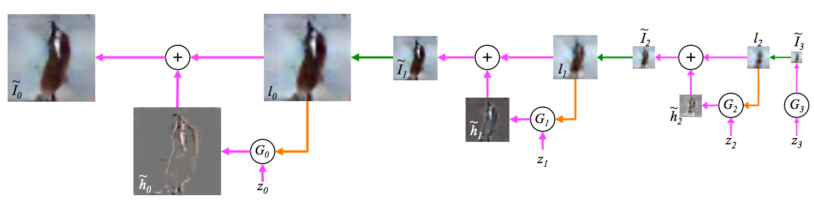
Figure 1: The sampling procedure for our LAPGAN model.
We start with a noise sample \(z_3\) (right side) and use a generative model \(G_3\) to generate \(\tilde{I}_3\).
This is upsampled (green arrow) and then used as the conditioning variable (orange arrow) \(l_2\) for the generative model at the next level, \(G_2\).
Together with another noise sample \(z_2\), \(G_2\) generates a difference image \(\tilde{h}_2\) which is added to \(l_2\) to create \(\tilde{I}_2\).
This process repeats across two subsequent levels to yield a final full resolution sample \(\tilde{I}_0\).
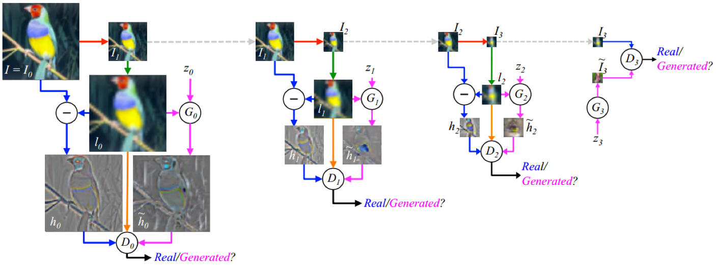
Figure 2: The training procedure for our LAPGAN model.
Starting with a 64x64 input image \(I\) from our training set (top left):
we take \(I_0 = I\) and blur and downsample it by a factor of two (red arrow) to produce \(I_1\);
we upsample \(I_1\) by a factor of two (green arrow), giving a low-pass version \(l_0\) of \(I_0\);
with equal probability we use \(l_0\) to create either a real or a generated example for the discriminative model \(D_0\).
In the real case (blue arrows), we compute high-pass \(h_0 = I_0 − l_0\) which is input to \(D_0\) that computes the probability of it being real vs generated.
In the generated case (magenta arrows), the generative network \(G_0\) receives as input a random noise vector \(z_0\) and \(l_0\). It outputs a generated high-pass image \(\tilde{h}_0 = G_0(z_0, l_0)\), which is input to \(D_0\).
In both the real/generated cases, \(D_0\) also receives \(l_0\) (orange arrow).
Optimizing Eqn. 2, \(G_0\) thus learns to generate realistic high-frequency structure \(\tilde{h}_0\) consistent with the low-pass image \(l_0\).
The same procedure is repeated at scales 1 and 2, using \(I_1\) and \(I_2\).
Note that the models at each level are trained independently.
At level 3, \(I_3\) is an 8×8 image, simple enough to be modeled directly with a standard GANs \(G_3\) & \(D_3\).