GRAN
Generating Images with Recurrent Adversarial Networks
Paper: https://arxiv.org/abs/1602.05110
Code: https://github.com/jiwoongim/GRAN
we propose a recurrent generative model that can be trained using adversarial training.
In order to quantitatively compare adversarial networks we also propose a new performance measure, that is based on letting the generator and discriminator of two models compete against each other.
Introduction
Currently, most common image generation models can be roughly categorized into two classes:
The first is based on probabilistic generative models, such as the variational autoencoder [11] and a variety of equivalent models introduced at the same time. The idea in these models is to train an autoencoder whose latent representation satisfies certain distributional properties, which makes it easy to sample from the hidden variables.
The second class of generative models is based on adversarial sampling [4]. This approach forgoes the need to encourage a particular latent distribution (and, in fact, the use of an encoder altogether), by training a simple feedforward neural network to generate “data-like” examples.
Motivated by the successes of sequential generation, in this paper, we propose a new image generation model based on a recurrent network.
we let the recurrent network learn the optimal procedure by itself.
we obtain very good samples without resorting to an attention mechanism and without variational training criteria (such as a KL-penalty on the hiddens).
we also introduce a new evaluation scheme based on a “cross-over” battle between the discriminators and generators of the two models.
Background
Model
We propose sequential modeling using GANs on images.
There is a close relationship between sequential generation and Backpropgating to the Input (BI). BI is a well-known technique where the goal is to obtain a neural network input that minimizes a given objective function derived from the network.
In this work, we explore a generative recurrent adversarial network as an intermediate between DRAW and gradient-based optimization based on a generative adversarial objective function.
Generative Recurrent Adversarial Networks
The main difference between GRAN versus other generative adversarial models is that the generator
G consists of a recurrent feedback loop that takes a sequence of noise samples drawn from the prior distribution \(z \sim p(z)\) and draws an output at multiple time steps \(\Delta C_1, \Delta C_2, \cdots, \Delta C_T\).
At each time step, \(t\), a sample \(z\) from the prior distribution is passed to a function \(f(·)\) along with the hidden states \(h_{c,t}\).
\(h_{c,t}\) represent the hidden state, or in other words, a current encoded status of the previous drawing \(\Delta C_{t−1}\).
\(\Delta C_t\) represents the output of the function \(f(·)\).
the function \(g(·)\) can be seen as a way to mimic the inverse of the function \(f(·)\).
the function \(f(·)\) acts as a decoder that receives the input from the previous hidden state \(h_{c,t}\) and noise sample \(z\), and function \(g(·)\) acts as an encoder that provides a hidden representation of the output \(\Delta C_{t−1}\) for time step \(t\).
\[z_t \sim p(Z)\]
\[h_{c,t} = g(\Delta C_{t−1})\]
\[h_{z,t} = \tanh(W z_t + b)\]
\[\Delta C_t = f([h_{z,t}, h_{c,t}])\]
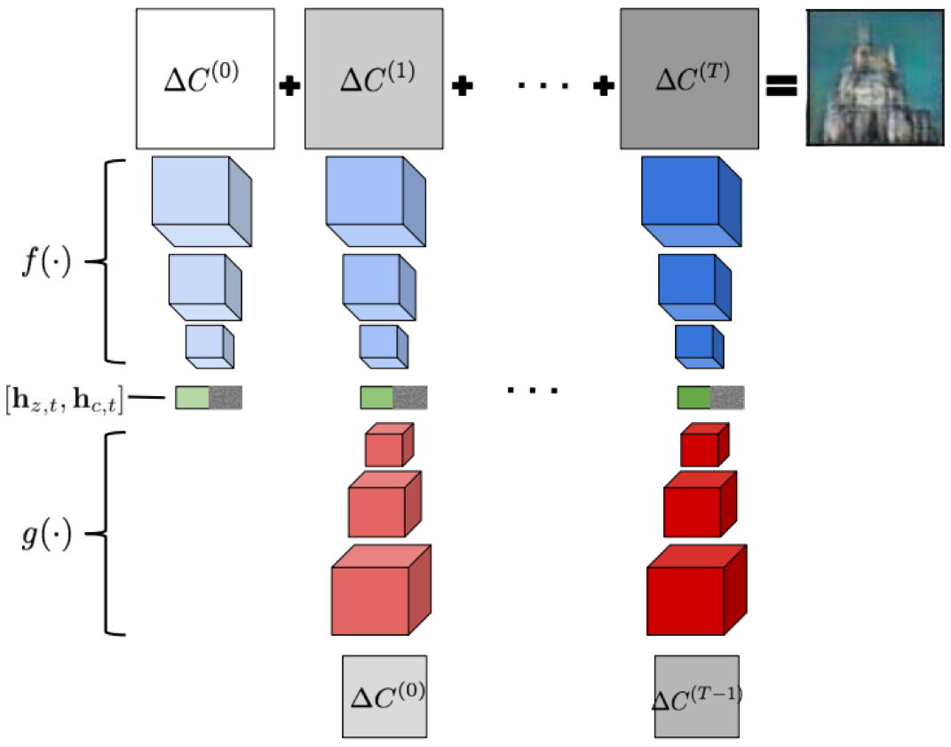
Figure 3. Abstraction of Generative Recurrent Adversarial Networks. The function \(f\) serves as the decoder and the function \(g\) serves as the encoder of GRAN.
Model Evaluation: Battle between GANs
Our approach is to directly compare two generative adversarial models by having them engage in a "battle" against each other.
In the training phase, \(G_1\) competes with \(D_1\) in order to be trained for the battle in the test phase.
In the test phase, model \(M_1\) plays against model \(M_2\) by having \(G_1\) try to fool \(D_2\) and vice-versa.
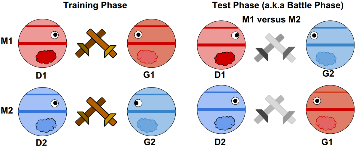
Figure 4. Training Phase of Generative Adversarial Networks.
At test time, we can look at the following ratios between the discriminative scores of the two models:
\[r_{test} \stackrel{def}{=} \frac{\epsilon (D_1(x_{test}))}{\epsilon (D_2(x_{test}))}\]
\[r_{sample} \stackrel{def}{=} \frac{\epsilon (D_1(G_2(z)))}{\epsilon (D_2(G_1(z)))}\]
where \(\epsilon(·)\) is the classification error rate, and \(x_{test}\) is the predefined test set.