Deeplab-Semi
(ICCV 2015) Weakly- and Semi-Supervised Learning of a Deep Convolutional Network for Semantic Image Segmentation
Paper: http://www.cv-foundation.org/openaccess/content_iccv_2015/papers/Papandreou_Weakly-_and_Semi-Supervised_ICCV_2015_paper.pdf
Project Page: http://liangchiehchen.com/projects/DeepLab_Models.html
Code: https://bitbucket.org/deeplab/deeplab-public/
提出使用图像级别标签或bounding box来进行弱监督或半监督学习语义分割。
基础网络是Deeplab,对只有图像级别标签的,使用EM去弱监督指导分割(E步骤:对每个位置的预测结果,若有该图像级别标签,则加上预设定的潜在参数\(b_l\))。
Bbox-Rect: 使用bbox里的像素作为分割的正样本(重叠时选面积最小的bbox)。
Bbox-Seg:使用DenseCRF预处理bbox的前景和背景(中心区域a%的像素为前景),前景标上bbox的标签。
Bbox-EM-Fixed:使用EM去精细化估计的分割图。
We study the more challenging problem of learning DCNNs for semantic image segmentation from either (1) weakly annotated training data such as bounding boxes or image-level labels or (2) a combination of few strongly labeled and many weakly labeled images, sourced from one or multiple datasets.
We develop Expectation-Maximization (EM) methods for semantic image segmentation model training under these weakly supervised and semi-supervised settings.
Introduction
A key bottleneck in building this class of DCNN-based segmentation models is that they typically require pixel-level annotated images during training.
According to [24], collecting bounding boxes around each class instance in the image is about 15 times faster/cheaper than labeling images at the pixel level.
Most existing approaches for training semantic segmentation models from this kind of very weak labels use multiple instance learning (MIL) techniques.
We develop novel online Expectation-Maximization (EM) methods for training DCNN semantic segmentation models from weakly annotated data.
Contributions
We present EM algorithms for training with image-level or bounding box annotation, applicable to both the weakly-supervised and semi-supervised settings.
We show that our approach achieves excellent performance when combining a small number of pixel-level annotated images with a large number of image-level or bounding box annotated images, nearly matching the results achieved when all training images have pixel-level annotations.
We show that combining weak or strong annotations across datasets yields further improvements. In particular, we reach 73.9% IOU performance on PASCAL VOC 2012 by combining annotations from the PASCAL and MS-COCO datasets.
Related work
Proposed Methods
We build on the DeepLab model for semantic image segmentation proposed in [5].
We encode the set of image-level labels by \(z\), with \(z_l = 1\), if the \(l\)-th label is present anywhere in the image.
Pixel-level annotations
In the fully supervised case illustrated in Fig. 1, the objective function is
\[J(\theta) = \log P(y \mid x; \theta) = \sum_{m = 1}^M \log P(y_m \mid x; \theta)\]
Image-level annotations
When only image-level annotation is available, we can observe the image values \(x\) and the image-level labels \(z\), but the pixel-level segmentations \(y\) are latent variables. We have the following probabilistic graphical model:
\[P(x, y, z; \theta) = P(x) \left(\Pi_{m = 1}^M P(y_m \mid x; \theta) \right) P (z \mid y)\]
We pursue an EM-approach in order to learn the model parameters \(\theta\) from training data.
the expected complete-data log-likelihood given the previous parameter estimate \(\theta '\) is
\[Q(\theta; \theta ') = \sum_y P(y \mid x, z; \theta ') \log P(y \mid x; \theta) \approx \log P(\hat{y} \mid x; \theta)\]
where we adopt a hard-EM approximation, estimating in the E-step of the algorithm the latent segmentation by
\[\begin{align*} \hat{y} & = \operatorname*{argmax}_y P(y \mid x; \theta ') P(z \mid y) \\ & = \operatorname*{argmax}_y \log P(y \mid x; \theta ') + \log P(z \mid y) \\ & = \operatorname*{argmax}_y \left(\sum_{m = 1}^M f_m(y_m \mid x; \theta ') + \log P(z \mid y) \right) \\ \end{align*}\]
In the M-step of the algorithm, we optimize \(Q(\theta; \theta ')\) by mini-batch SGD similarly to (1), treating \(\hat{y}\) as ground truth segmentation.
EM-Fixed
\[\hat{y}_m = \operatorname*{argmax}_{y_m} \hat{f_m}(y_m) = f_m (y_m \mid x; \theta ') + \phi (y_m, z)\]
We assume that
\[\phi(y_m = l, z) = \begin{cases} b_l & \text{if} z_l = 1 \\ 0 & \text{if} z_l = 0 \end{cases}\]
We set the parameters \(b_l = b_{fg}\), if \(l > 0\) and \(b_0 = b_{bg}\), with \(b_{fg} > b_{bg} > 0\).
EM-Adapt
we assume that \(\log P(z \mid y) = \phi(y, z) + (\text{const})\), where \(\phi(y, z)\) takes the form of a cardinality potential [23, 32, 35]. In particular, we encourage at least a \(\rho_l\) portion of the image area to be assigned to class \(l\), if \(z_l = 1\), and enforce that no pixel is assigned to class \(l\), if \(z_l = 0\). We set the parameters \(\rho_l = \rho_{fg}\), if \(l > 0\) and \(\rho_0 = \rho_{bg}\).
EM vs. MIL
While this approach (MIL) has worked well for image classification tasks [28, 29], it is less suited for segmentation as it does not promote full object coverage.
Bounding Box Annotations
Bbox-Rect
amounts to simply considering each pixel within the bounding box as positive example for the respective object class.
Ambiguities are resolved by assigning pixels that belong to multiple bounding boxes to the one that has the smallest area.
Bbox-Seg
The bounding boxes fully surround objects but also contain background pixels that contaminate the training set with false positive examples for the respective object classes.
we perform automatic foreground/background segmentation.
we use the same CRF as in DeepLab. More specifically, we constrain the center area of the bounding box (\(\alpha \%\) of pixels within the box) to be foreground, while we constrain pixels outside the bounding box to be background.
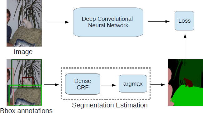
Figure 3. DeepLab model training from bounding boxes. (Bbox-Seg)
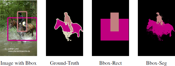
Figure 4. Estimated segmentation from bounding box annotation.
Bbox-EM-Fixed
an EM algorithm that allows us to refine the estimated segmentation maps throughout training. The method is a variant of the EMFixed algorithm in Sec. 3.2, in which we boost the present foreground object scores only within the bounding box area.
Mixed strong and weak annotations
we bundle to each mini-batch a fixed proportion of strongly/weakly annotated images, and employ our EM algorithm in estimating at each iteration the latent semantic segmentations for the weakly annotated images.
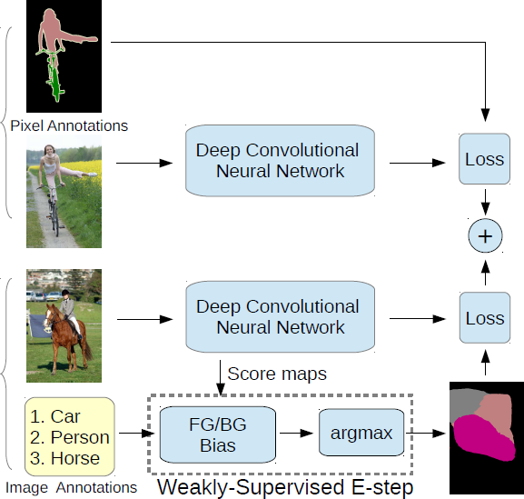
Figure 5. DeepLab model training on a union of full (strong labels) and image-level (weak labels) annotations.
Experimental Evaluation
Experimental Protocol
Datasets
PASCAL VOC 2012 segmentation benchmark
20 foreground object classes and one background class.
1464 (train), 1449 (val), and 1456 (test) images for training, validation, and test
10582 (train aug) and 12031 (trainval aug) images.
MS-COCO 2014
123287 images in its trainval set.
80 foreground object classes and one background class
Reproducibility
Weak annotations
The image-level labels are easily generated by summarizing the pixel-level annotations
the bounding box annotations are produced by drawing rectangles tightly containing each object instance (PASCAL VOC 2012 also provides instance-level annotations)
Network architectures
two DCNN architectures of [5], with parameters initialized from the VGG-16 ImageNet [11] pretrained model of [34]
large FOV (224×224), small FOV (128×128)
Training
We employ our proposed training methods to learn the DCNN component of the DeepLab-CRF model of [5]. For SGD, we use a mini-batch of 20-30 images and initial learning rate of 0.001 (0.01 for the final classifier layer), multiplying the learning rate by 0.1 after a fixed number of iterations. We use momentum of 0.9 and a weight decay of 0.0005. Fine-tuning our network on PASCAL VOC 2012 takes about 12 hours on a NVIDIA Tesla K40 GPU.
Pixel-level annotations
Image-level annotations
| Method | #Strong | #Weak | val IOU |
|---|---|---|---|
| EM-Fixed (Weak) | - | 10,582 | 20.8 |
| EM-Adapt (Weak) | - | 10,582 | 38.2 |
| EM-Fixed (Semi) | 200 | 10,382 | 47.6 |
| EM-Fixed (Semi) | 500 | 10,082 | 56.9 |
| EM-Fixed (Semi) | 750 | 9,832 | 59.8 |
| EM-Fixed (Semi) | 1,000 | 9,582 | 62.0 |
| EM-Fixed (Semi) | 1,464 | 5,000 | 63.2 |
| EM-Fixed (Semi) | 1,464 | 9,118 | 64.6 |
| Strong | 1,464 | - | 62.5 |
| Strong | 10,582 | - | 67.6 |
Table 1. VOC 2012 val performance for varying number of pixel-level (strong) and image-level (weak) annotations (Sec. 4.3).
| Method | #Strong | #Weak | test IOU |
|---|---|---|---|
| MIL-FCN | - | 10k | 25.7 |
| MIL-sppxl | - | 760k | 35.8 |
| MIL-obj | BING | 760k | 37.0 |
| MIL-seg | MCG | 760k | 40.6 |
| EM-Adapt (Weak) | - | 12k | 39.6 |
| EM-Fixed (Semi) | 1.4k | 10k | 66.2 |
| EM-Fixed (Semi) | 2.9k | 9k | 68.5 |
| Strong | 12k | - | 70.3 |
Table 2. VOC 2012 test performance for varying number of pixel-level (strong) and image-level (weak) annotations (Sec. 4.3).
Bounding box annotations
| Method | #Strong | #Box | val IOU |
|---|---|---|---|
| Bbox-Rect (Weak) | - | 10,582 | 52.5 |
| Bbox-EM-Fixed (Weak) | - | 10,582 | 54.1 |
| Bbox-Seg (Weak) | - | 10,582 | 60.6 |
| Bbox-Rect (Semi) | 1,464 | 9,118 | 62.1 |
| Bbox-EM-Fixed (Semi) | 1,464 | 9,118 | 64.8 |
| Bbox-Seg (Semi) | 1,464 | 9,118 | 65.1 |
| Strong | 1,464 | - | 62.5 |
| Strong | 10,582 | - | 67.6 |
Table 3. VOC 2012 val performance for varying number of pixel-level (strong) and bounding box (weak) annotations (Sec. 4.4).
| Method | #Strong | #Box | test IOU |
|---|---|---|---|
| BoxSup | MCG | 10k | 64.6 |
| BoxSup | 1.4k (+MCG) | 9k | 66.2 |
| Bbox-Rect (Weak) | - | 12k | 54.2 |
| Bbox-Seg (Weak) | - | 12k | 62.2 |
| Bbox-Seg (Semi) | 1.4k | 10k | 66.6 |
| Bbox-EM-Fixed (Semi) | 1.4k | 10k | 66.6 |
| Bbox-Seg (Semi) | 2.9k | 9k | 68.0 |
| Bbox-EM-Fixed (Semi) | 2.9k | 9k | 69.0 |
| Strong | 12k | - | 70.3 |
Table 4. VOC 2012 test performance for varying number of pixel-level (strong) and bounding box (weak) annotations (Sec. 4.4).
Exploiting Annotations Across Datasets
Qualitative Segmentation Results
Conclusions
The paper has explored the use of weak or partial annotation in training a state of art semantic image segmentation model. Extensive experiments on the challenging PASCAL VOC 2012 dataset have shown that:
Using weak annotation solely at the image-level seems insufficient to train a high-quality segmentation model.
Using weak bounding-box annotation in conjunction with careful segmentation inference for images in the training set suffices to train a competitive model.
Excellent performance is obtained when combining a small number of pixel-level annotated images with a large number of weakly annotated images in a semi-supervised setting, nearly matching the results achieved when all training images have pixel-level annotations.
Exploiting extra weak or strong annotations from other datasets can lead to large improvements.